White Papers
Quantum Computing · White Paper · 2026

Letting Physics
Do the Computation

Understanding the Role of Quantum Computers in Modern Computing

Quantum computing is often portrayed as a revolutionary technology capable of replacing classical computers across a wide range of tasks. While quantum processors offer advantages for certain problem classes, this narrative obscures a more fundamental insight: computation is deeply tied to the physical systems used to implement it. This paper examines computation from a physical perspective and demonstrates how some problems are solved more naturally when the computational process is embedded directly in the physics of the system — through mechanical sorting and Grover's quantum search algorithm.

By Viren Patel — Quantum Computing

Published: 2026 ~20 min read 2 Interactive Simulations
SHA-256: 40A2D1B0C6A984378D38C1C2816F5CB59A4BA19970B32A11EED3C79FE5646866

Note: This whitepaper presents conceptual and simulation-based analysis for educational purposes. Interactive demonstrations were built to illustrate quantum algorithm mechanics and physical computation principles.

Scroll to explore
01

Introduction

Why the history of computing is inseparable from the physics of its implementation

Key Takeaways

  • 1The history of computing is inseparable from the physical systems used to implement it
  • 2Mechanical, analog, and digital computers each excelled because their structure matched their problems
  • 3Quantum computers are specialized, not universal — they exploit quantum mechanical behavior for specific problem classes
  • 4Understanding computation as a physical process is essential to understanding quantum advantage
  • 5The future is an ecosystem of specialized machines, not a single dominant architecture

Computing Paradigms

EraMechanismStrength
MechanicalGears & leversArithmetic
AnalogElectrical circuitsDifferential equations
DigitalBinary logicGeneral-purpose
QuantumQubit evolutionSuperposition problems

In recent years, quantum computing has emerged as a new computational paradigm based on the principles of quantum mechanics. Popular discussions often describe quantum computers as dramatically faster replacements for classical machines. While quantum processors can provide advantages for certain tasks, the idea that they will broadly replace classical computers is misleading.

Quantum computers are not general-purpose accelerators for all forms of computation. Instead, they represent specialized systems that exploit quantum mechanical behavior to efficiently represent and evolve certain classes of problems. Understanding this distinction requires examining computation not only as an abstract algorithmic process, but as a physical process implemented by real systems.

Key Insight

Quantum computers are not general-purpose accelerators. They are specialized systems that exploit quantum mechanical behavior for specific problem classes. The same was true of every computational paradigm that came before: each excelled because its physical structure aligned naturally with the problems it was designed to solve.

02

Computation as a Physical Process

How physical dynamics can perform computation without symbolic algorithms

Most discussions of algorithms focus on symbolic manipulation and logical operations performed by digital machines. However, computation can also emerge directly from the dynamics of physical systems.

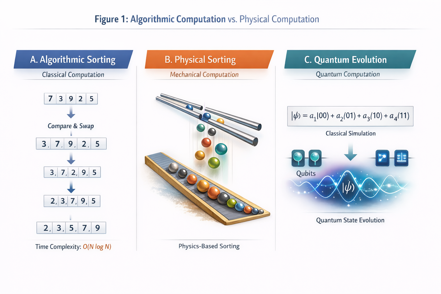
Consider the task of sorting objects by size. In a classical computer, sorting requires algorithms that repeatedly compare elements and rearrange their positions in memory. Even highly optimized algorithms require a sequence of discrete comparisons and data movements.

An alternative approach is to design a physical system whose natural dynamics perform the sorting. In the mechanical sorting device illustrated below, marbles of different diameters are placed between two initially touching parallel rods. The rods gradually separate while remaining parallel, creating a continuously increasing gap. When the gap becomes slightly larger than the diameter of a marble, that marble falls through — no measurement or algorithmic comparison required. The ordering emerges directly from the geometry and motion of the system.
Algorithmic Computation vs. Physical Computation
Click to zoom
Figure 1

Algorithmic vs. Physical Computation

Classical sorting uses compare-and-swap. Physical sorting uses geometry. Quantum evolution extends the principle further — the physics of the system performs the computation.

Physical Computation

The sorting rule is encoded directly in the physical constraints of the device. No measurements or algorithmic comparisons are required. The physics of the system performs the computation — sorting emerges from geometry.

⚙️ Interactive Demonstration

The physical sorting mechanism can be explored through an interactive simulation. Marbles of varying diameters are placed between two parallel rods that gradually separate. As the gap increases, smaller marbles fall first — demonstrating how computation can arise from physical dynamics rather than symbolic operations.
⚙️
Physical Sorting Demonstration Interactive simulation — marbles, parallel rods, physics-driven sorting
03

The Landscape of Computing Machines

A diverse ecosystem of architectures, each optimized for different problem classes

🖥️

CPU

Sequential logic and control tasks. General-purpose, programmable, handles branching and I/O efficiently.

GPU / TPU

Massively parallel numerical workloads. Scientific computing, machine learning, and neural network inference.

⚛️

Quantum Processor

Qubits evolving under quantum mechanics. Superposition, interference, and entanglement for specific problem classes.

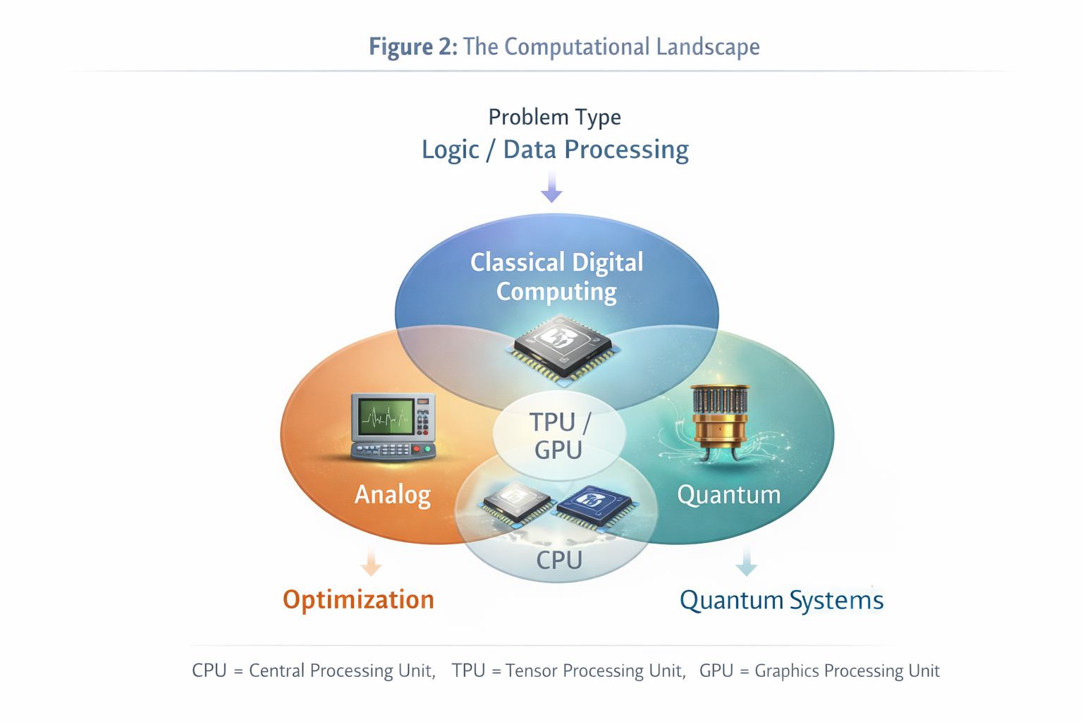
Modern computing systems consist of a diverse ecosystem of architectures optimized for different classes of problems. Each architecture excels in domains where its underlying physical structure aligns naturally with the computational task. Recognizing this diversity is essential for understanding the role of quantum computers within the future of computing.

The Computational Landscape
Click to zoom
Figure 2

The Computational Landscape

Classical Digital, Analog, GPU/TPU, and Quantum computing — each occupying a distinct niche defined by the physical principles it exploits.

04

The Exponential Wall of Classical Simulation

Why classical computers cannot efficiently simulate quantum systems beyond ~50 qubits

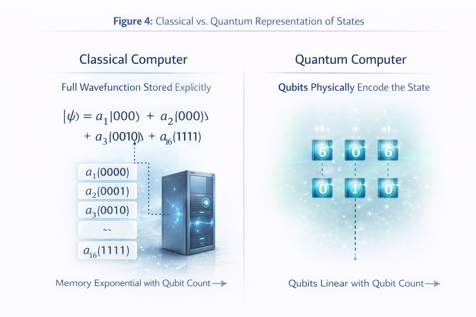
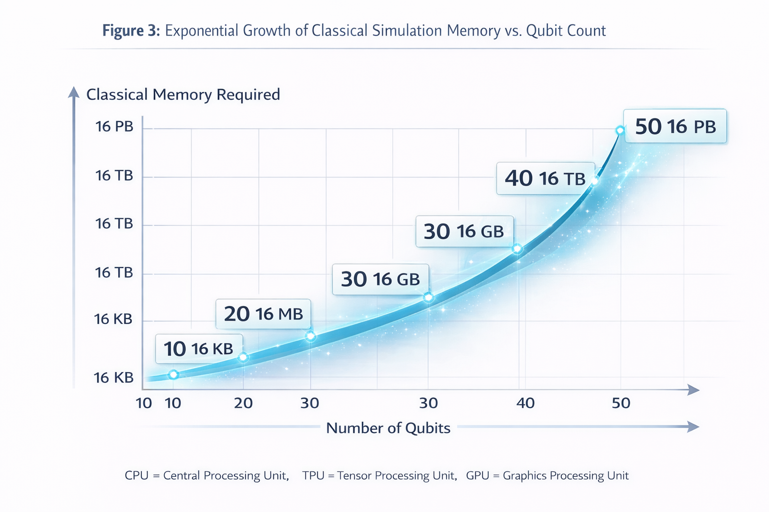
One of the most challenging problems in classical computing is the simulation of quantum systems. The state of a quantum system is described by a wavefunction, which contains the amplitudes of all possible configurations. For a system of $n$ qubits, the complete quantum state contains $2^n$ complex amplitudes. A classical computer must explicitly store and manipulate this exponentially growing state vector.

Exponential Memory Growth
Click to zoom
Figure 3

Exponential Memory Growth vs. Qubit Count

Classical simulation memory grows as $2^n$ complex amplitudes. 50 qubits already exceeds 16 petabytes — beyond any classical system.

Exponential Scaling

10 qubits: 16 KB  |  20 qubits: 16 MB  |  30 qubits: 16 GB

40 qubits: 16 TB  |  50 qubits: 16 PB — beyond any classical machine

10 qubits
16 KB
20 qubits
16 MB
30 qubits
16 GB
40 qubits
16 TB
50 qubits
16 PB
05

Quantum Representation of Information

How quantum processors encode exponential state spaces in linear physical resources

Classical Simulation

Stores the entire wavefunction explicitly in memory.

Memory required = 2n × 16 bytes
n = 30 → 16 GB classical RAM

Quantum Processor

Encodes the state physically within qubit registers.

Physical qubits required = n
n = 30 → 30 physical qubits

A register of $n$ qubits naturally represents a quantum state containing $2^n$ amplitudes. Quantum operations manipulate these qubits according to the principles of quantum mechanics, allowing the system to evolve as a physical quantum process rather than as a numerical simulation. The state exists physically within the qubit system itself — no explicit memory needed.

Classical vs Quantum Representation
Click to zoom
Figure 4

Classical vs. Quantum State Representation

Classical: memory grows exponentially ($2^n$ amplitudes stored). Quantum: physical qubits scale linearly — $n$ qubits encode $n$-qubit states natively.

Classical vs. Quantum

Classical: Memory grows exponentially with qubit count ($2^n$ complex amplitudes stored explicitly).

Quantum: Physical qubits scale linearly — $n$ qubits naturally encode $n$-qubit states through their physical evolution.

06

Quantum Search & Amplitude Amplification

Grover's algorithm: from $O(N)$ to $O(\sqrt{N})$ through constructive quantum interference

While quantum computers do not accelerate every computational task, they can provide advantages for certain types of problems. One example is Grover's search algorithm, which enables searching an unsorted database of $N$ elements in approximately $\sqrt{N}$ steps rather than the $N$ steps required classically.

The key mechanism is amplitude amplification. Rather than sequentially checking each candidate solution, Grover's algorithm prepares a quantum superposition of all possible states and iteratively amplifies the probability amplitude of the correct solution through constructive interference. An oracle marks the target state by flipping its phase, followed by a diffusion operation that redistributes amplitudes across the state space.

Grover's Speedup

Classical search: $O(N)$ steps  |  Quantum search: $O(\sqrt{N})$ steps

For $N = 1{,}000{,}000$: Classical needs ~1M checks, Quantum needs ~1,000

6.1  Quantum Oracles and the Role of Classical Functions

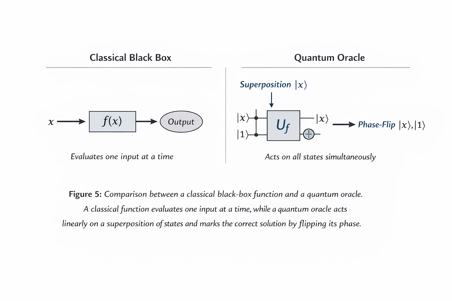
A common misconception is that Grover's algorithm evaluates a classical function across all inputs simultaneously. In reality, a purely classical black box cannot operate on a quantum superposition — interacting with it would collapse the quantum state. Instead, Grover's algorithm requires a quantum implementation of the function, known as an oracle circuit.

The oracle performs a reversible transformation, applying a phase flip to the target state while leaving all others unchanged. Mathematically:

$$U_f |x\rangle = (-1)^{f(x)} |x\rangle$$

where $f(x) = 1$ for the target state and $0$ for all others. This phase flip is unobservable by itself, but sets up conditions for constructive interference in subsequent iterations.

Classical Black Box vs Quantum Oracle
Click to zoom
Figure 5

Classical Black Box vs. Quantum Oracle

A classical function evaluates one input at a time. A quantum oracle acts linearly on a superposition and marks the correct solution by phase inversion.

Why the Oracle Must Be Reversible

All quantum operations must be reversible — no information can be destroyed. A classical function that outputs 0 or 1 is irreversible. To use it within Grover's algorithm, it must be translated into a reversible quantum circuit using phase kickback, where an ancilla qubit enables the oracle to imprint the function's result as a phase on the input register.

The Real Cost of Grover's Algorithm

Grover's algorithm provides a quadratic reduction in oracle evaluations: $O(\sqrt{N})$ vs $O(N)$. However, the actual computational cost is $O(\sqrt{N} \times C)$, where $C$ is the cost of one oracle circuit execution.

MetricComplexity
Classical search$O(N)$ oracle evaluations
Grover search$O(\sqrt{N})$ oracle evaluations
Actual runtime$O(\sqrt{N} \times$ cost of oracle circuit$)$
Key Insight

Grover's algorithm does not "search all possibilities simultaneously." It manipulates the quantum wavefunction so that interference gradually concentrates probability on the correct answer. The oracle marks — it does not find. The diffusion operator amplifies.

6.2  Geometric Interpretation of Grover's Algorithm

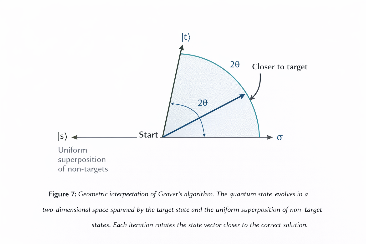
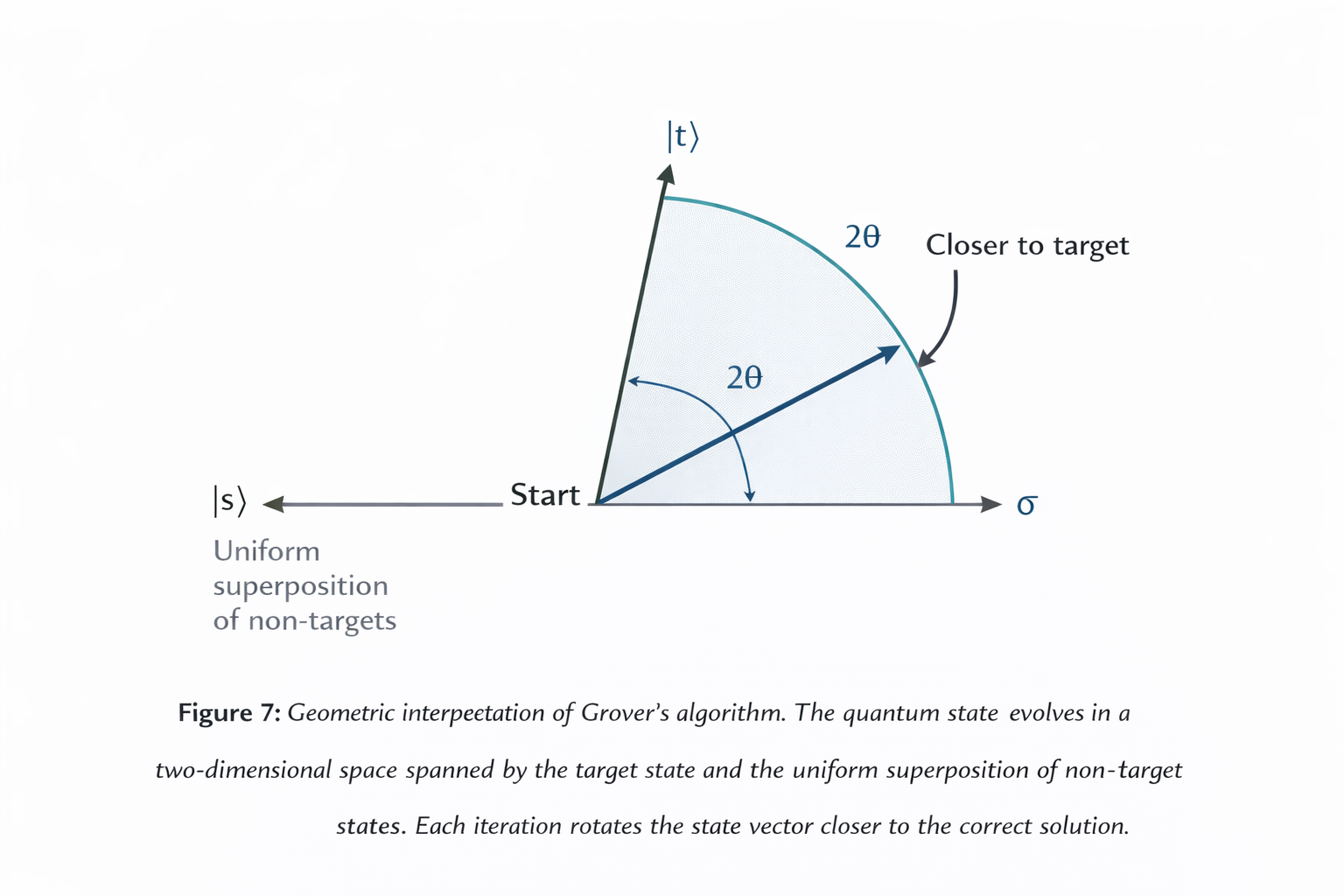
The dynamics of Grover's algorithm can be understood through an elegant geometric interpretation. The entire computation takes place within a two-dimensional subspace spanned by two orthogonal vectors: the target state and the uniform superposition of all non-target states.

Each Grover iteration performs a rotation by a fixed angle of $2\theta$ towards the target state. After approximately $\frac{\pi}{4}\sqrt{N}$ iterations, the state vector aligns with the target, maximizing the measurement probability.

Geometric Interpretation of Grover's Algorithm
Click to zoom
Figure 7

Geometric Interpretation

The quantum state evolves in a 2D space: target $|t\rangle$ vs. non-target superposition $|s\rangle$. Each iteration rotates the state vector by $2\theta$ closer to the solution.

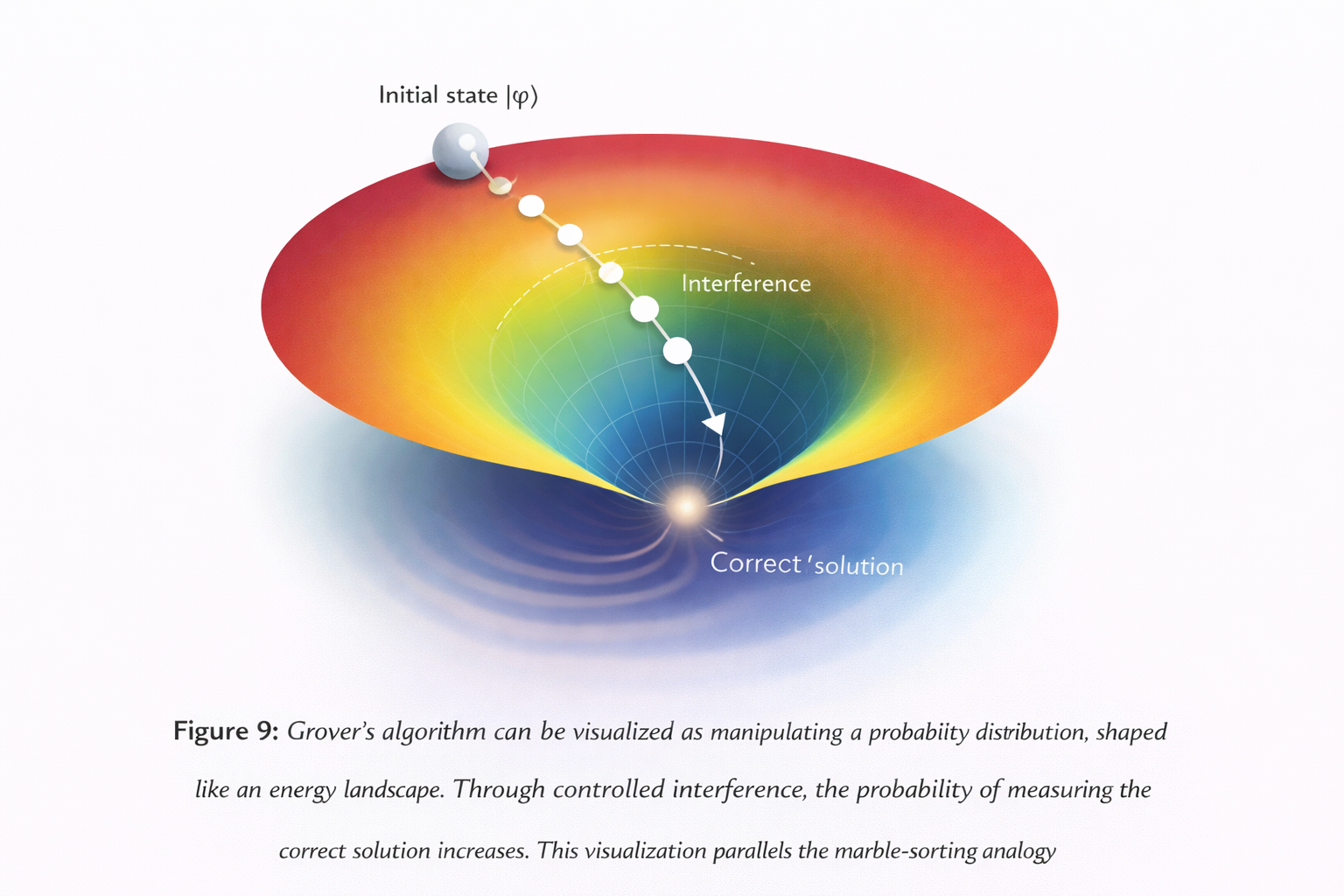
Energy Landscape Visualization
Click to zoom
Figure 8

Energy Landscape Visualization

Controlled interference guides the wavefunction toward the solution — just as gravity guides marbles in the physical sorting device. The correct answer sits at the bottom of a probability funnel.

Geometric Insight

The oracle reflects the state about the non-target subspace (phase flip). The diffusion operator reflects about the mean amplitude. Together, these two reflections produce a rotation toward the target state.

07

Interactive Simulations & Visualization

Making the abstract mathematics of amplitude amplification directly observable

To develop physical intuition for the mechanisms behind Grover's algorithm, an interactive simulation was built that visualizes three key representations simultaneously: the amplitude distribution across all basis states, the geometric rotation in the two-dimensional Grover subspace, and the evolving probability distribution over successive iterations.

Interactive Grover Simulation Screenshot
Click to zoom
Figure 9

Interactive Grover Algorithm Simulation

The simulation displays the quantum circuit, amplitude bars, geometric rotation panel, and probability evolution simultaneously. Fully interactive — step through oracle and diffusion operations.

Simulation Panels

  • Top panel — Quantum circuit: oracle & diffusion ops
  • Left panel — Amplitude distribution of all basis states
  • Center panel — Geometric rotation in 2D subspace
  • Right panel — Probability distribution over iterations

Interactive Features

  • Change number of qubits (scales search space)
  • Choose target state
  • Step through oracle and diffusion individually
  • Toggle math mode & learning mode
⚛️
Grover's Algorithm Visualization Adjustable qubits · Step-by-step oracle & diffusion · Real-time amplitude & probability charts

7.1  Insights from Building the Simulation

Several observations became clearer through the process of building the simulation. The geometric interpretation of Grover's algorithm is far more intuitive when visualized as a rotation in a two-dimensional subspace than when described purely through matrix algebra.

The oracle does not find the answer. It only flips the phase of the marked state, which by itself produces no observable change. The diffusion operator is the component responsible for amplification through interference, reflecting all amplitudes about their mean so that the marked state gains amplitude at the expense of the others.

Simulation Insights

The oracle marks — it does not find. The diffusion operator amplifies. Together they produce a rotation: each iteration brings the state closer to the target. After $\frac{\pi}{4}\sqrt{N}$ steps, measurement yields the answer.

08

Hybrid Computational Architectures

The realistic vision: classical and quantum processors working in concert

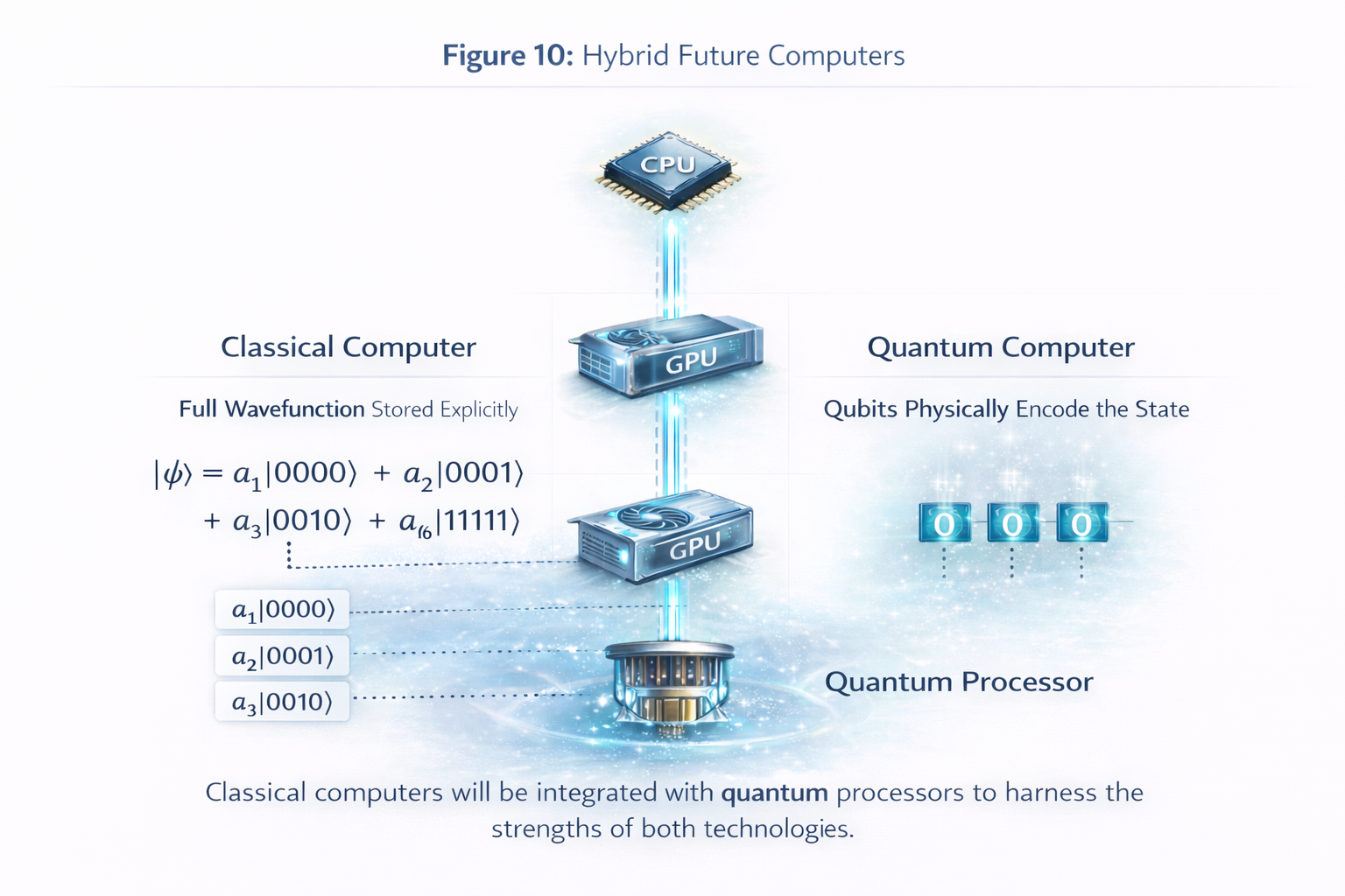
The most realistic vision for the future of computing is not one in which quantum computers replace classical machines. Instead, future systems will likely combine multiple specialized processors within a unified architecture. Classical processors will orchestrate the overall computation. GPUs and classical accelerators will continue to serve large-scale numerical workloads. Quantum processors will be invoked selectively for operations that exploit superposition and interference — acting as specialized accelerators rather than replacements.

Hybrid Future Computer Architecture
Click to zoom
Figure 10

Hybrid Future Computer Architecture

Classical CPUs orchestrate the workflow. GPUs handle parallel numerical workloads. Quantum processors execute operations that exploit superposition and interference for specific problem classes.

Hybrid Framework: Best of All Architectures

🖥️

Classical CPU

Orchestrates workflow, handles branching logic, I/O, and general-purpose computation

GPU / TPU

Massively parallel numerical workloads: ML training, scientific simulation, linear algebra

⚛️

Quantum Processor

Selectively invoked for superposition & interference — search, optimization, quantum simulation

09

Conclusion

An ecosystem of specialized machines, each leveraging the physics best suited to its problems

Quantum computers represent an important extension of the computational landscape, but they should not be viewed as universal replacements for classical machines. By examining computation from a physical perspective, we see that different computational architectures arise from different underlying physical systems.

Mechanical systems can perform sorting through geometry. Classical digital computers perform symbolic manipulation through logical operations. Quantum processors exploit interference and superposition to evolve complex state spaces. Each paradigm is powerful precisely because its physical structure aligns with the problems it solves.

The future of computing will therefore not be defined by a single dominant architecture, but by an ecosystem of specialized machines, each designed to leverage the physical principles best suited to the problems they solve.

Central Thesis

The future of computing is not about one architecture replacing another. It is about an ecosystem of specialized machines, each leveraging the physical principles best suited to the problems they solve.

Acknowledgment

The author would like to acknowledge the IQM School of Quantum Computing for providing a structured and rigorous introduction to quantum computing concepts. The lectures and educational resources offered through the program were instrumental in shaping the foundational perspective presented in this paper. The clarity of the curriculum helped establish a solid conceptual understanding of quantum systems, quantum algorithms, and the physical principles that distinguish quantum computation from classical approaches. This acknowledgment reflects sincere appreciation for the quality and accessibility of the program.

10

References

Foundational publications and further reading

[1]
Feynman, R. P. — Simulating Physics with Computers. International Journal of Theoretical Physics, 21(6/7), 467–488, 1982.
[2]
Grover, L. K. — A Fast Quantum Mechanical Algorithm for Database Search. Proceedings of the 28th Annual ACM Symposium on Theory of Computing, pp. 212–219, 1996.
[3]
Nielsen, M. A. & Chuang, I. L. — Quantum Computation and Quantum Information. Cambridge University Press, 10th Anniversary Edition, 2010.
[4]
Aaronson, S. — Quantum Computing Since Democritus. Cambridge University Press, 2013.